healpy is a Python module that allows to call the HEALPix library from Python. These libraries contain a series of methods to deal with producing skymaps, with special focus on CMB plotting. In particular, it includes two way conversion between pixel-wise data of a skymap and the corresponding \(a_{\ell m}\) coefficients, as well as two way conversion between \(a_{\ell m}\) coefficients and \(C_\ell\) coefficients. This makes it a great tool to numerically deal with some of the quantitites introduced in the previous section without having to program a lot yourself, as well as to explore visually the appearance of different spherical harmonics of power spectra.

Here, you'll get introduced to the basic functionality of healpy, but first you need to make sure that you have it installed in your Python environment. You can do that with the usual pip install healpy, conda install healpy or whatever method is convenient for your Python environment. To check this is working, you can start a clean Python notebook and type import healpy as hp.

1 - Imports and spherical harmonics convention

For the following exercise, you'll also need numpy mostly to use arrays that are recognized y healpy, and scipy to load the spherical harmonics. Then, you can start your code with import healpy as hp import numpy as np import scipy.special The spherical harmonics are defined for being solutions to a linear differential equation. Then, multiplication by a constant of a solution to the equation is also a solution. This introduces several possible conventions about what that constant is. Here, we use the spherical harmonics defined such that $$Y_l^m(\theta,\phi)=\sqrt{\frac{2\ell+1}{4\pi}\frac{(\ell-m)!}{(\ell+m)!}}P_\ell^m(\cos\theta)e^{i m\phi},$$ where the \(P_\ell^m\) are the associated Legendre polynomials, and \(\theta\in[0,\pi]\), \(\phi\in[02\pi)\), \(\ell\in\mathbb N\) and \(m\in\mathbb Z\) such that \(|m|\leq\ell\). The spherical harmonics defined inside scipy use a strange convention. The function template is scipy.special.sph_harm(m, n, theta, phi, out=None), and it calculates $$Y_n^m(\theta,\phi)=\sqrt{\frac{2n+1}{4\pi}\frac{(n-m)!}{(n+m)!}}P_n^m(\cos\phi)e^{i m\theta}.$$ One can see that the roles of \(\theta\) and \(\phi\) are reversed, and that \(\ell\) is renamed to \(n\). Moreover, the order of arguments is unusual. One would usually read \(Y_\ell^m(\theta,\phi)\) as “y l m of theta and phi”. The order in the scipy implementation would correspond to “y m l of phi and theta”. In order to avoid confusion, one can define the following function: def Y(l,m,theta,phi) : return scipy.special.sph_harm(m,l,phi,theta)

2 - Basics of healpy maps

The difficulty in making skymaps is related to that of tessellation. One is interested in filling an elliptical shape with smaller shapes, each of them of one color, at specific locations. This is one of the functions that healpy does for you. To do so, one of the elementary quantities that define a healpy skymap is the number of these elementary shapes that will fill up the ellipse. This is indeed specified by a different variable, usually referred to as nside in the healpy documentation. 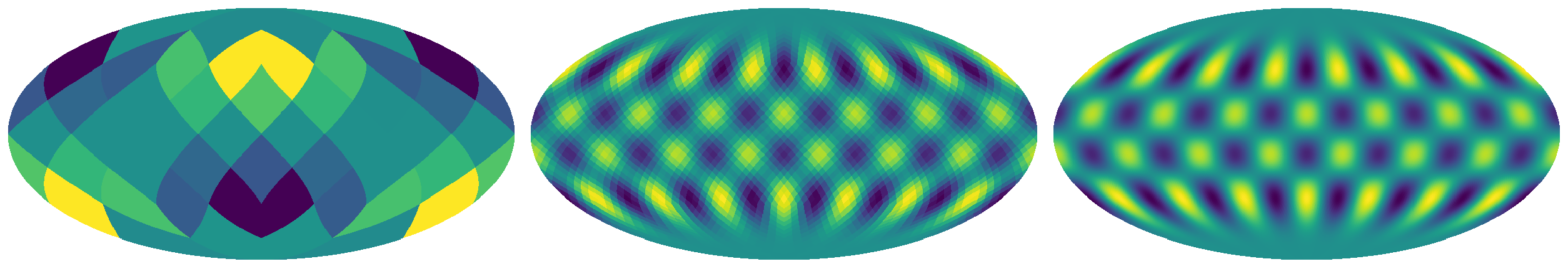As they mention there, it seems conventional to use a power of 2 for this variable. Here you can see two examples of skymaps produced by healpy with a value of nside of 2 (left), 16 (middle) and 128 (right). This choice affects output resolution and computation efficiency. For testing, lower numbers may be more convenient, while for publication you may want a number so large that the individual shapes are not discernible.

Since nside is a variable that is passed to each function that makes a map, it is convenient to define a global value for it at the beginning of your script or notebook, rather than manually writing it each time. The code below serves as a definition of a global variable NSIDE, and includes a little script that allows you to see the actual number of pixels that would be in the map, as well as the angular resolution corresponding to your choice. In this example, I make NSIDE be \(2^6=64\). NSIDE=2**6 print( "Maps with NSIDE {} have {} pixels, offering a resolution of is {:.2} deg".format( NSIDE, hp.nside2npix(NSIDE),hp.nside2resol(NSIDE, arcmin=True) / 60 ) ) The actual, pixel-wise information that is plotted in a map is, by default, stored in a numpy.ndarray one-dimensional object, with as many entries as pixels are on the map. The number of pixels on a map with a given value of nside can be obtained with the healpy function hp.nside2npix. Then, once you decide on the value of NSIDE, any array that has a length equal to hp.nside2npix(NSIDE) can be represented on a skymap. The items in the array are plotted in order, starting at the north pole (\(\theta=0\)) and going down from left to right. You can do a simple example by plotting an array with the natural numbers in order, as shown in the example below. Once you have an array that you are ready to use to create a map, simply call the healpy function to do so: mollview (note that this uses a Mollweide projection; other options are possible). NPIX = hp.nside2npix(NSIDE) x = np.arange(NPIX) hp.mollview(x)

3 - Plotting functions on a skymap

One of the potential applications of healpy is to make a color plot of a given function that depends on two angular coordinates \(f(\theta,\phi)\). In order to do so, the function must be evaluated at all values of \(\theta\) and \(\phi\) that correspond to one of the pixels in the skymap. The conversion between pixels and coordinates is not trivial, but healpy does it for you. Once NSIDE is specified, the relation between them is fixed, and can be easily evaluated using the healpy function pix2ang. This function provides two numpy.ndarray objects, with the values \(\theta_i\) of \(\phi_i\) corresponding to the i-th pixel, respectively. This function requires us to provide the pixels we are interested in: we may want the values of \(\theta\) and \(\phi\) for a single pixel, for a few of them, or for all of them. This is passed as the second argument to pix2ang. In the example below, I want all pixels, so I make an array of all pixel numbers using NPIX from before: allpixels = np.arange(NPIX) theta, phi = hp.pix2ang(NSIDE, allpixels) I could use then the values of theta and phi to evaluate an arbitrary function and make a map. While there are more direct ways of doing this, an option would be to initialize an empty array of the right size, and fill the elements one by one. Here, I do so to make a plot of the function \(f(\theta,\phi)=\sin(2\theta)\cos(5\phi)\): def fun(th,ph): return np.sin(2*th)*np.cos(5*ph) array = np.empty(NPIX) for i in range(NPIX): array[i] = fun(theta[i],phi[i]) hp.mollview(array)

4 - Plotting spherical harmonics

To make a plot of a specific spherical harmonic, you could use the spherical harmonic function defined above, which ultimately comes from scipy. One may be interested in plotting not a single spherical harmonic, but a combination of them. Due to the properties of spherical harmonics, any (smooth? what are the requirements?) function defined on the sphere can be written as a linear combination of spherical harmonics. This expansion usually expressed in the following way $$f(\theta,\phi)=\sum_{\ell=0}^\infty\sum_{m=-\ell}^\ell a_{\ell m}Y_\ell^m(\theta,\phi).$$

It may be that you're interested in plotting a given function \(f\) for which you already know the values of the \(a_{\ell m}\) coefficients. If that's not the case, and instead you have an actual functional dependence like in the example shown above, go ahead and use that method. But if you actually have the values of the \(a_{\ell m}\) you don't need to program your function \(f\) on Python following the equation above. Rather, healpy has you covered. If you give it the values of the coefficients \(a_{\ell m}\), healpy is able to calculate the corresponding function on its own, which can be used to make a map of it.

Just like the pixels have to be ordered in a specific way for the mollview function to understand them, the same is true for the list of \(a_{\ell m}\) coefficients. Usually, the function one wants to plot is a real function, but you can see how the spherical harmonics are complex. In order to guarantee the reality of \(f(\theta,\phi)\) in the expression above, it must be real for every value of \(\ell\) (since the spherical harmonics are independent for different values of it). Then, $$\sum_{m=-\ell}^\ell a_{\ell m}Y_\ell^m(\theta,\phi)$$ must be real. This is achieved by cancelling out the contributions of a given value of \(m\) with its negative, since combinations like \(e^{im\phi}+e^{-im\phi}\) are real. You can see how this condition becomes \(a_{\ell -m}=a^*_{\ell m}\), so the coefficients with negative \(m\) are uniquely determined from those with positive \(m\). This means that in order to specify the expansion of a real function in terms of spherical harmonics one doesn't need to provide the coefficients with negative \(m\) separately; those with \(m=0,1,\dots,\ell\) will suffice.

In general, this means that for each \(\ell\), one must provide \(\ell+1\) coefficients \(a_{\ell m}\). Generally, spherical harmonics with larger values of \(\ell\) oscillate faster with the angle \(\theta\). Therefore, a map of higher resolution would be necessary to capture all the features of spherical harmonics with very large \(\ell\). By the same token, if one is not planning on making a very high resolution plot, because it will be printed on a paper, one doesn't need to include all the spherical harmonics with very large \(\ell\), as they will only add computation time without any noticeable result. For this reason, healpy assumes that the (in principle) infinite sum that defines a function in terms of the spherical harmonics is truncated, so that it is instead $$f(\theta,\phi)=\sum_{\ell=0}^{\ell_\mathrm{max}}\sum_{m=-\ell}^\ell a_{\ell m}Y_\ell^m(\theta,\phi).$$

With all this in mind, the way healpy expects the \(a_{\ell m}\) coefficients to be passed is as an ordered list of finite size, in which the elements are ordered as follows: first, list the coefficients with \(m=0\) for all values of \(\ell\in[0,\ell_\mathrm{max}]\), then do the same for \(m=1\), and so on. The list would look as follows: $$[a_{00},a_{10},\dots,a_{\ell_\mathrm{max} 0},a_{11},a_{21},\dots,a_{\ell_\mathrm{max},1},\dots,a_{\ell_\mathrm{max}\ell_\mathrm{max}}].$$ Notice the fact that there is never a coefficient with \(m\gt\ell\), so after one is done listing all coefficients with \(m=0\), the first one with \(m=1\) doesn't have \(\ell=0\) but \(\ell=1\).

Some of the functions included in healpy will help you keep track of all the coefficients that are required. For instance, you can find the number of coefficients needed once you specify \(\ell_\mathrm{max}\) with the healpy function Alm.getsize. Also, once you specify the value of \(\ell_\mathrm{max}\) healpy can tell you the values of \(\ell\) and \(m\) that correspond to a specific position in the list of \(a_{\ell m}\) coefficients. This is done by means of the function Alm.getlm. You can see a usage example of both below: LMAX = 3 almsize = hp.Alm.getsize(LMAX) print("For l_max={}, you need {} coefficients:".format(LMAX,almsize)) for i in range(almsize): print("For i={}, (l,m)={}".format(i,hp.Alm.getlm(LMAX,i))) Similarly, you may be interested in knowing what is the position in the array of \(a_{\ell m}\) coefficients that corresponds to a specific choice of \((\ell,m)\). To do so, you can use the healpy function Alm.getidx. Of course, the position depends on the maximum number \(\ell_\mathrm{max}\), so you need to pass this as an argument. For example, imagine you want to assign the value \(1.5\) to the coefficient \(a_{3,2}\), when we are considering \(\ell_\mathrm{max}=3\), like the example above. Then you could do the following: alm = np.empty(almsize) pos = hp.Alm.getidx(LMAX,3,2) alm[pos] = 1.5

Finally, imagine that you want to define a value for all coefficients \(a_{\ell m}\) following an analytic expression for them. Let's choose \(\ell_\mathrm{max}=30\), and implement the coefficients \(a_{\ell m}=\sin(\ell+m)/(2\ell+1)\), independent of \(m\): LMAX = 30 almsize = hp.Alm.getsize(LMAX) alm = np.empty(almsize,dtype="complex128") def almfun(l,m) : return np.sin(m+l)/(2*l+1) for i in range(almsize): l,m = hp.Alm.getlm(LMAX,i) alm[i] = almfun(l,m) Notice that the array of \(a_{\ell m}\) has to be created as a complex variable. Otherwise, healpy will have problems making a map out of it.

Finally, we can create the map that corresponds to this choice of \(a_{\ell m}\) coefficients. This is achieved with the alm2map function of healpy. From a list of coefficients, it creates an array formatted in the exact way that is required to produce a map. This can be passed to the function mollview like before, to produce the desired output: map = hp.alm2map(alm,NSIDE) hp.mollview(map, title="Combination of Ylms")